Asymptotic Analysis

As we know that data structure is a way of organizing the data efficiently and that efficiency is measured either in terms of time or space. So, the ideal data structure is a structure that occupies the least possible time to perform all its operation and the memory space. Our focus would be on finding the time complexity rather than space complexity, and by finding the time complexity, we can decide which data structure is the best for an algorithm.

The main question arises in our mind that on what basis should we compare the time complexity of data structures?. The time complexity can be compared based on operations performed on them. Let's consider a simple example.

Suppose we have an array of 100 elements, and we want to insert a new element at the beginning of the array. This becomes a very tedious task as we first need to shift the elements towards the right, and we will add new element at the starting of the array.

Suppose we consider the linked list as a data structure to add the element at the beginning. The linked list contains two parts, i.e., data and address of the next node. We simply add the address of the first node in the new node, and head pointer will now point to the newly added node. Therefore, we conclude that adding the data at the beginning of the linked list is faster than the arrays. In this way, we can compare the data structures and select the best possible data structure for performing the operations.

How to find the Time Complexity or running time for performing the operations?

The measuring of the actual running time is not practical at all. The running time to perform any operation depends on the size of the input. Let's understand this statement through a simple example.

Suppose we have an array of five elements, and we want to add a new element at the beginning of the array. To achieve this, we need to shift each element towards right, and suppose each element takes one unit of time. There are five elements, so five units of time would be taken. Suppose there are 1000 elements in an array, then it takes 1000 units of time to shift. It concludes that time complexity depends upon the input size.

Therefore, if the input size is n, then f(n) is a function of n that denotes the time complexity.

How to calculate f(n)?

Calculating the value of f(n) for smaller programs is easy but for bigger programs, it's not that easy. We can compare the data structures by comparing their f(n) values. We can compare the data structures by comparing their f(n) values. We will find the growth rate of f(n) because there might be a possibility that one data structure for a smaller input size is better than the other one but not for the larger sizes. Now, how to find f(n).

Let's look at a simple example.

f(n) = 5n² + 6n + 12

where n is the number of instructions executed, and it depends on the size of the input.

When n=1

% of running time due to 5n² = * 100 = 21.74%

% of running time due to 6n = * 100 = 26.09%

% of running time due to 12 = * 100 = 52.17%

From the above calculation, it is observed that most of the time is taken by 12. But, we have to find the growth rate of f(n), we cannot say that the maximum amount of time is taken by 12. Let's assume the different values of n to find the growth rate of f(n).

As we can observe in the above table that with the increase in the value of n, the running time of 5n² increases while the running time of 6n and 12 also decreases. Therefore, it is observed that for larger values of n, the squared term consumes almost 99% of the time. As the n² term is contributing most of the time, so we can eliminate the rest two terms.

Therefore,

f(n) = 5n²

Here, we are getting the approximate time complexity whose result is very close to the actual result. And this approximate measure of time complexity is known as an Asymptotic complexity. Here, we are not calculating the exact running time, we are eliminating the unnecessary terms, and we are just considering the term which is taking most of the time.

In mathematical analysis, asymptotic analysis of algorithm is a method of defining the mathematical boundation of its run-time performance. Using the asymptotic analysis, we can easily conclude the average-case, best-case and worst-case scenario of an algorithm.

It is used to mathematically calculate the running time of any operation inside an algorithm.

Example: Running time of one operation is x(n) and for another operation, it is calculated as f(n2). It refers to running time will increase linearly with an increase in 'n' for the first operation, and running time will increase exponentially for the second operation. Similarly, the running time of both operations will be the same if n is significantly small.

Usually, the time required by an algorithm comes under three types:

Worst case: It defines the input for which the algorithm takes a huge time.

Average case: It takes average time for the program execution.

Best case: It defines the input for which the algorithm takes the lowest time

Asymptotic Notations

The commonly used asymptotic notations used for calculating the running time complexity of an algorithm is given below:

• Big oh Notation (?)
• Omega Notation (Ω)
• Theta Notation (θ)

Big oh Notation (O)

• Big O notation is an asymptotic notation that measures the performance of an algorithm by simply providing the order of growth of the function.
• This notation provides an upper bound on a function which ensures that the function never grows faster than the upper bound. So, it gives the least upper bound on a function so that the function never grows faster than this upper bound.

It is the formal way to express the upper boundary of an algorithm running time. It measures the worst case of time complexity or the algorithm's longest amount of time to complete its operation. It is represented as shown below: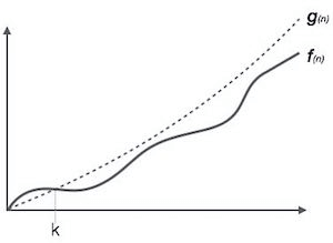

For example:

If f(n) and g(n) are the two functions defined for positive integers,

then f(n) = O(g(n)) as f(n) is big oh of g(n) or f(n) is on the order of g(n)) if there exists constants c and no such that:

f(n)≤c.g(n) for all n≥no

This implies that f(n) does not grow faster than g(n), or g(n) is an upper bound on the function f(n). In this case, we are calculating the growth rate of the function which eventually calculates the worst time complexity of a function, i.e., how worst an algorithm can perform.

Let's understand through examples

Example 1: f(n)=2n+3 , g(n)=n

Now, we have to find Is f(n)=O(g(n))?

To check f(n)=O(g(n)), it must satisfy the given condition:

f(n)<=c.g(n)

First, we will replace f(n) by 2n+3 and g(n) by n.

2n+3 <= c.n

Let's assume c=5, n=1 then

2*1+3<=5*1

5<=5

For n=1, the above condition is true.

If n=2

2*2+3<=5*2

7<=10

For n=2, the above condition is true.

We know that for any value of n, it will satisfy the above condition, i.e., 2n+3<=c.n. If the value of c is equal to 5, then it will satisfy the condition 2n+3<=c.n. We can take any value of n starting from 1, it will always satisfy. Therefore, we can say that for some constants c and for some constants n0, it will always satisfy 2n+3<=c.n. As it is satisfying the above condition, so f(n) is big oh of g(n) or we can say that f(n) grows linearly. Therefore, it concludes that c.g(n) is the upper bound of the f(n). It can be represented graphically as: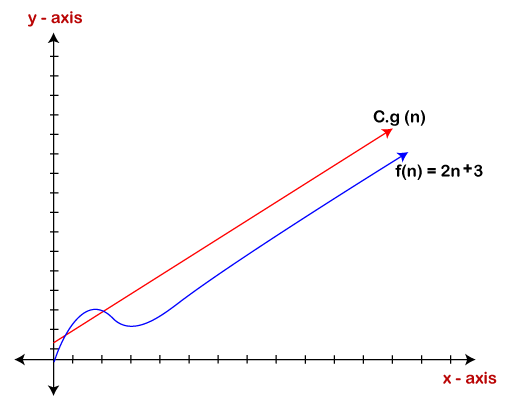

The idea of using big o notation is to give an upper bound of a particular function, and eventually it leads to give a worst-time complexity. It provides an assurance that a particular function does not behave suddenly as a quadratic or a cubic fashion, it just behaves in a linear manner in a worst-case.

Omega Notation (Ω)

• It basically describes the best-case scenario which is opposite to the big o notation.
• It is the formal way to represent the lower bound of an algorithm's running time. It measures the best amount of time an algorithm can possibly take to complete or the best-case time complexity.
• It determines what is the fastest time that an algorithm can run.

If we required that an algorithm takes at least certain amount of time without using an upper bound, we use big- Ω notation i.e. the Greek letter "omega". It is used to bound the growth of running time for large input size.

If f(n) and g(n) are the two functions defined for positive integers,

then f(n) = Ω (g(n)) as f(n) is Omega of g(n) or f(n) is on the order of g(n)) if there exists constants c and no such that:

f(n)>=c.g(n) for all n≥no and c>0

Let's consider a simple example.

If f(n) = 2n+3, g(n) = n,

Is f(n)= Ω (g(n))?

It must satisfy the condition:

f(n)>=c.g(n)

To check the above condition, we first replace f(n) by 2n+3 and g(n) by n.

2n+3>=c*n

Suppose c=1

2n+3>=n (This equation will be true for any value of n starting from 1).

Therefore, it is proved that g(n) is big omega of 2n+3 function.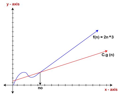

As we can see in the above figure that g(n) function is the lower bound of the f(n) function when the value of c is equal to 1. Therefore, this notation gives the fastest running time. But, we are not more interested in finding the fastest running time, we are interested in calculating the worst-case scenarios because we want to check our algorithm for larger input that what is the worst time that it will take so that we can take further decision in the further process.

Theta Notation (θ)

• The theta notation mainly describes the average case scenarios.
• It represents the realistic time complexity of an algorithm. Every time, an algorithm does not perform worst or best, in real-world problems, algorithms mainly fluctuate between the worst-case and best-case, and this gives us the average case of the algorithm.
• Big theta is mainly used when the value of worst-case and the best-case is same.
• It is the formal way to express both the upper bound and lower bound of an algorithm running time.

Let's understand the big theta notation mathematically:

Let f(n) and g(n) be the functions of n where n is the steps required to execute the program then:

f(n)= θg(n)

The above condition is satisfied only if when

c1.g(n)<=f(n)<=c2.g(n)

where the function is bounded by two limits, i.e., upper and lower limit, and f(n) comes in between. The condition f(n)= θg(n) will be true if and only if c1.g(n) is less than or equal to f(n) and c2.g(n) is greater than or equal to f(n). The graphical representation of theta notation is given below: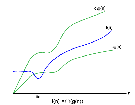

Let's consider the same example where
f(n)=2n+3
g(n)=n

As c1.g(n) should be less than f(n) so c1 has to be 1 whereas c2.g(n) should be greater than f(n) so c2 is equal to 5. The c1.g(n) is the lower limit of the of the f(n) while c2.g(n) is the upper limit of the f(n).

c1.g(n)<=f(n)<=c2.g(n)

Replace g(n) by n and f(n) by 2n+3

c1.n <=2n+3<=c2.n

if c1=1, c2=2, n=1

1*1 <=2*1+3 <=2*1

1 <= 5 <= 2 // for n=1, it satisfies the condition c1.g(n)<=f(n)<=c2.g(n)

If n=2

1*2<=2*2+3<=2*2

2<=7<=4 // for n=2, it satisfies the condition c1.g(n)<=f(n)<=c2.g(n)

Therefore, we can say that for any value of n, it satisfies the condition c1.g(n)<=f(n)<=c2.g(n). Hence, it is proved that f(n) is big theta of g(n). So, this is the average-case scenario which provides the realistic time complexity.

Why we have three different asymptotic analysis?

As we know that big omega is for the best case, big oh is for the worst case while big theta is for the average case. Now, we will find out the average, worst and the best case of the linear search algorithm.

Suppose we have an array of n numbers, and we want to find the particular element in an array using the linear search. In the linear search, every element is compared with the searched element on each iteration. Suppose, if the match is found in a first iteration only, then the best case would be Ω(1), if the element matches with the last element, i.e., nth element of the array then the worst case would be O(n). The average case is the mid of the best and the worst-case, so it becomes θ(n/1). The constant terms can be ignored in the time complexity so average case would be θ(n).

So, three different analysis provide the proper bounding between the actual functions. Here, bounding means that we have upper as well as lower limit which assures that the algorithm will behave between these limits only, i.e., it will not go beyond these limits.

Common Asymptotic Notations